

Introduction
Hello Actuarial Enthusiasts!!!
This article is about estimating the empirical one step and multi-step transition probabilities using Markov Chain and to build a rewards program for a large airline based on the travel miles. This article will give you an insight on the applications of Markov chain and how it is used in the real life to solve the real business problems using R.
This article is based on one of the CAST (Certificate in Actuarial Software Techniques) project. The project can be viewed from the link below:
The first step towards solving any business problem is to understand the problem in depth and what are the basic objectives to be achieved. So, let’s get started by understanding the problem first.
Given Data and the Problem:
We are given the data regarding the cumulative miles earned by each passenger, for 15000 such passengers. We want to use this data of last five years (From month 1 to month 60) to design a Rewards program based on the loyalty of the passengers (i.e. the more the miles covered, the more frequent flyer and loyal the passenger is, and hence more the reward) , which is categorized into 4 levels, namely:
- Level 1 – Bronze Level, 0 to 5000 miles
- Level 2 – Silver Level, 5001 to 12000 miles
- Level 3 – Gold Level, 12001 to 18000 miles
- Level 4 – Platinum Level, 18001 miles and above
Please download the data file from the project page given above or by clicking here.
Analysis of the Business Problem:
- Identifying Time Domain and State space
There are 4 states say State 0 (Bronze level), State 1 (Silver level), State 2 (Gold level) and State 3 (Platinum level). Hence, the state space of the process is discrete in nature.
Since the transitions are recorded month wise, hence the time domain of the process is discrete.
Also, the probability of moving from one state to the next, only depends on the current state and not on any of the previous states, thus, satisfying the Markov property.
Hence, the process is a Markov chain.
- Nature of the process
Also, since the process is cumulative in nature, it can only increase by one step i.e. from Bronze to silver, from silver to gold and from gold to platinum. It is also possible to remain in a particular level for consecutive months together. However, it is not possible to go back from a higher level to a lower level. Also, state 3 is the absorbing state as once a person reaches state 3, he remains there forever.
Objectives of the Business Problem:
The given data is to be converted into Markov chain considering the 4 states as defined above, and a model is to be generated to compute the one step and the multi-step probability of transition from one category to the other based on the data provided.
So, now, let’s proceed towards the second step in solving the business problem and to achieve the targeted objectives, i.e. dividing the business problem into smaller parts and start solving in R.
The problem of estimating the transition probabilities can be divided into 5 parts:
- Counting the number of singles
- Counting the number of doubles
- Calculating the one step transition probabilities
- Extending this further to calculating the multi-step transition probabilities
- Plotting the results for better visualization and for drawing conclusions
Part 1: Counting the number of singles
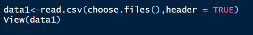
Step1: Open your RStudio and import the data file into R and name it as say, data1 and you can also view whether the data file is correctly imported or not by running the following code.
Step2:
Now, we need to count the number of singles i.e. ni’s which are defined as the no. of possible transitions out of each state ‘i’ (for each of these 15000 passengers) i.e.
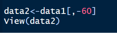
Ni= The number of times t such such that xt=i. Since it is the observed no. of transitions and not just the no. of times the process is in state ‘i’, we take the time from 1 to 59 and hence exclude the last column, as there is no completed transition out of the last state. This is done by:
The ni’s are then calculated, using the criteria defined above for the cumulative miles, for each state i=0,1,2,3 using the length function in R and the calculated values are then presented in the form of the table by making a data frame containing the number of singles i.e.
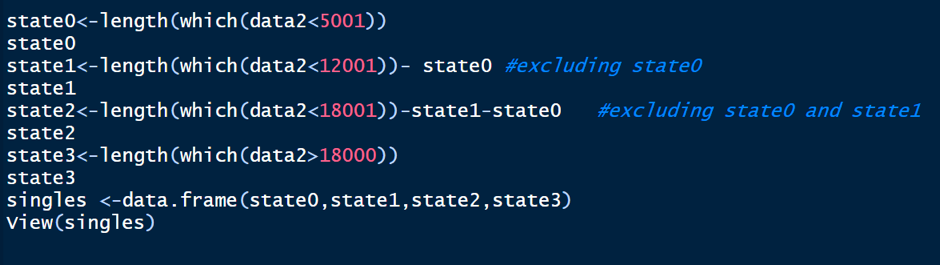
We will get the output of the created data frame singles as:

Hurray!!! we have successfully completed the 1st part of the problem.
Part 2: Counting the number of doubles
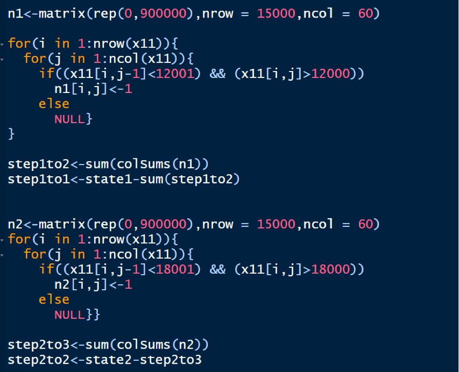
Now, we calculate the no. of possible transitions from state ‘i’, to state ‘j’, i.e. nij’s. Nij is defined as So, we first convert our original data into the matrix form and then count the number of doubles with the help of “for loop”, by displaying 1’s wherever the state changes from 0 to 1 in each column and then summing these sum of the Columns to get the total count of doubles. We run the following code:
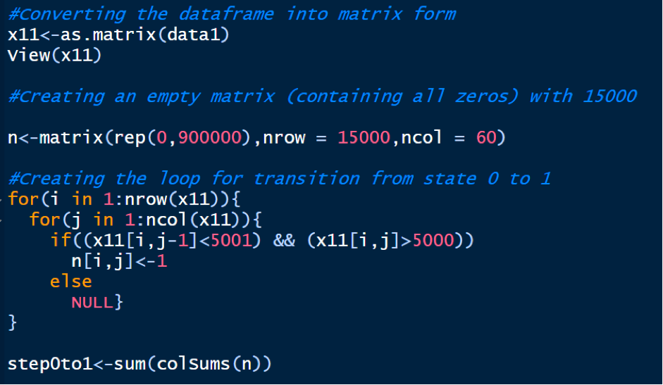
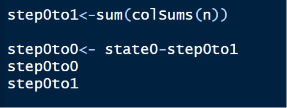
This is the total count of transitions from state 0 to 1. Now, the total count of transitions from state 0 to 0 is simply the total number of transitions out of state 0 minus the number of transitions from state 0 to 1 as either a process can remain in state 0 or moves to state 1.
Now, repeat the above process for states 1 and 2.
Since the state 3 is an absorbing state, as once the process reaches state 3, it cannot move out of state 3, so, only the transition of n33 is possible, which is simply the number of times, the process remains in state 3. Also, we finally, present our calculated nij’s in the form of a data frame.
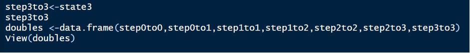
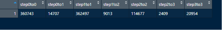
We finally get the output as:
Wooohoooo!!! We have completed the second part of this project successfully!!
Part 3: Calculating the one step transition probabilities
Since the process is Markov, we have:
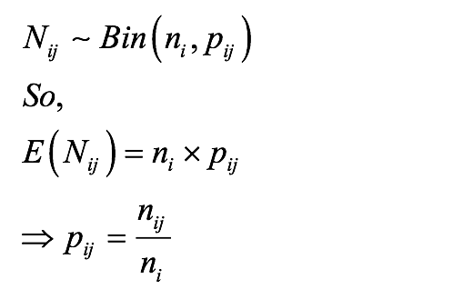
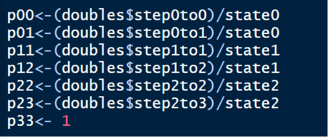
So, pij’s are calculated by extracting the nij from the data frame and dividing it by ni, as shown below:
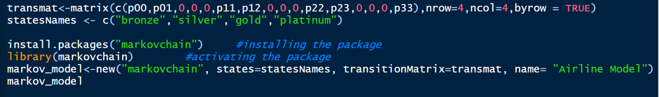
We, then create a transition matrix of these transition probabilities, and also, name the row and column names as the state names. We finally convert this into the Markov model by installing a package markov chain and activating it by running the following code:
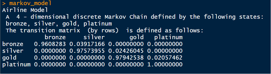
We finally, get the output of the Markov model generated and the one step transition probabilities as below:
We finally proceed to the part 4 by extending all this we have learnt to calculate the multi-step probabilities now.
Part 4: Calculating the multi-step transition probabilities
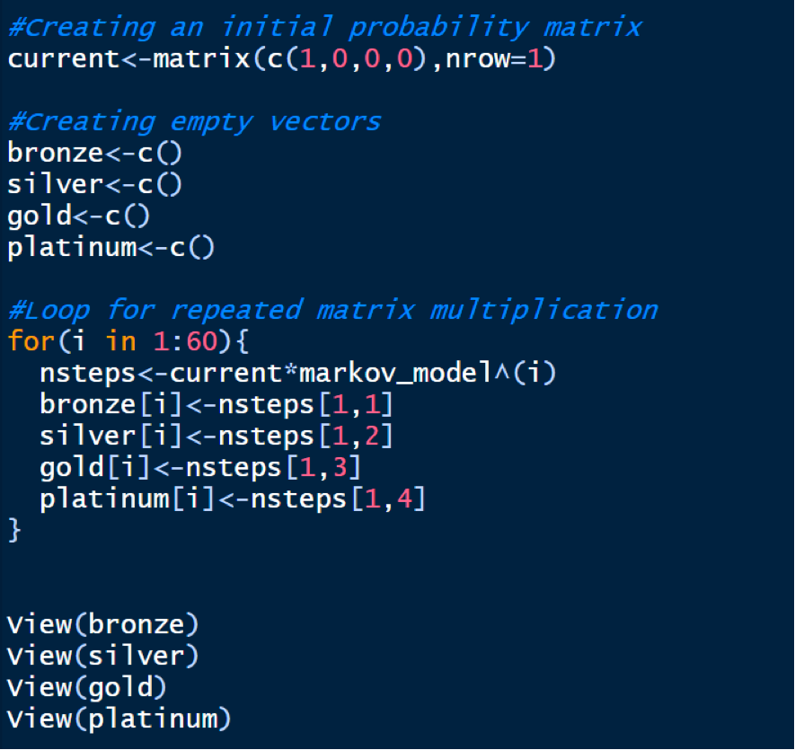
Let’s say we want to generate probabilities of being in any reward category at different times ranging from 1 to 60.
We start with defining the current or the initial state of any passenger. Since, the process always starts in state 0, the initial state of any new passenger is state 0 with probability 1. We then multiply this initial probability matrix (denoted by, say q) with the transition matrix obtained above (in part 3, denoted by say P) as many number of times as we want the probabilities for. For example, if we want the probabilities of being in each state after time 10, then q*(P10) will give the desired result. You can then view the probabilities for each state for different times ranging from 1 to 60. We do this in R, by running the following code:
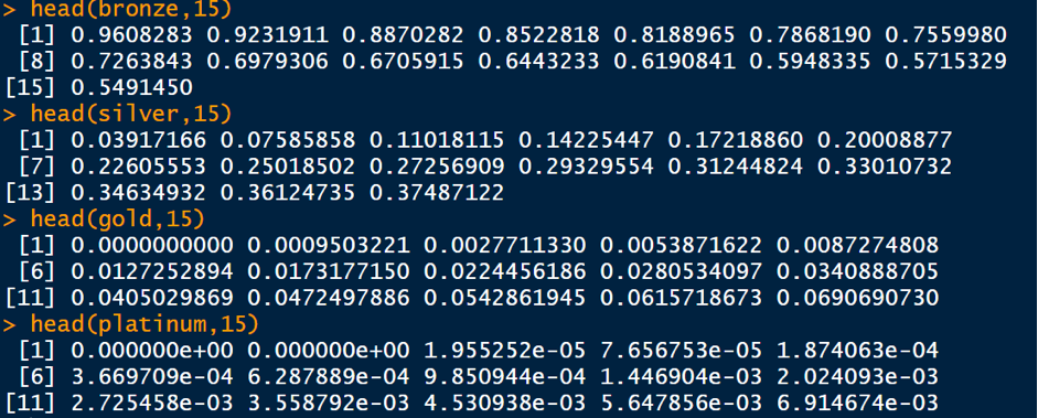
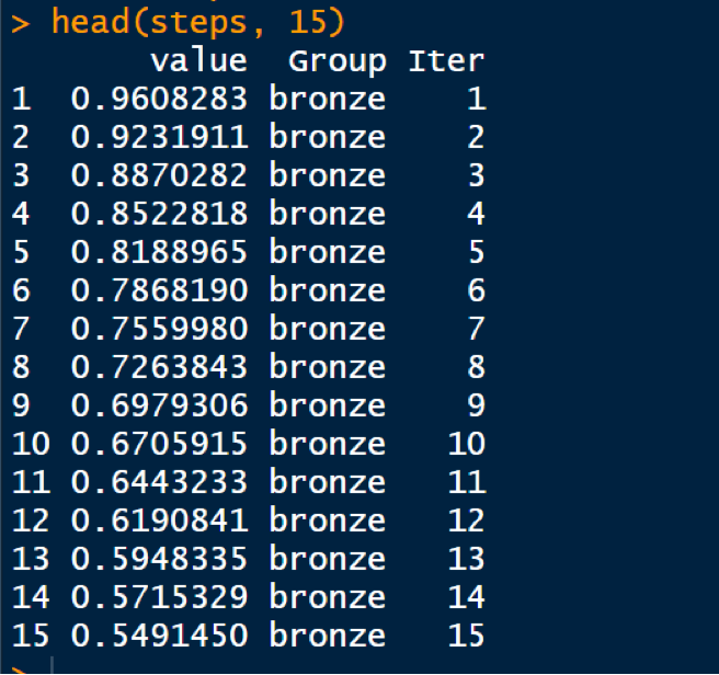
You can confirm, say the first 15 values of the multi-step probabilities by using the head function as:
Finally, let’s proceed to the final part in our project of creating a graph of these multi-step probabilities for data visualization and concluding the project.
Part 5: Plotting the multi-step transition probabilities
We use the “ggplot2” package in R for data visualization. You can learn more about this package by visiting the following links:
https://cran.r-project.org/web/packages/ggplot2/ggplot2.pdf
https://www.rdocumentation.org/packages/ggplot2/versions/3.3.2/topics/ggplot
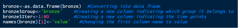
We convert all these multi step probabilities of each state into the data frame and then combine these various groups into a matrix for all the times 1 to 60 by running the following set of codes:
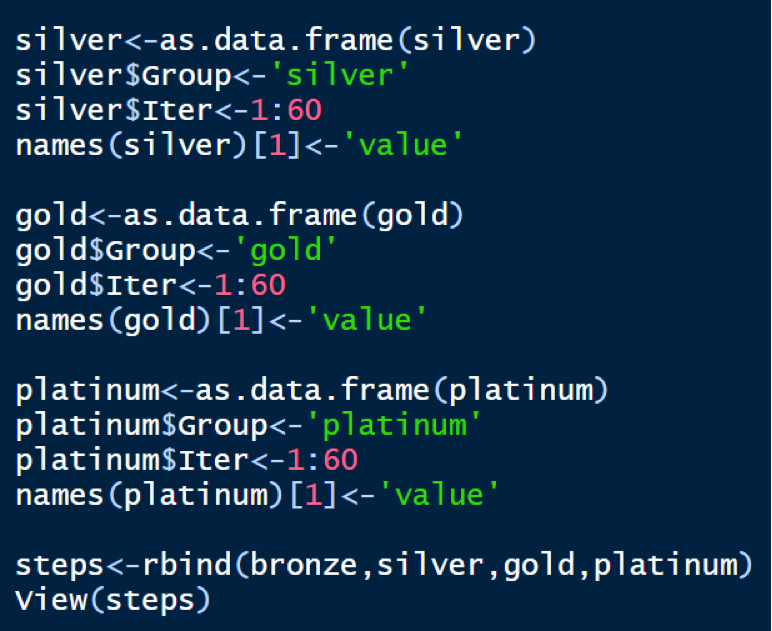
We repeat the same for other states and combine all states into the matrix form by:
You can confirm the output by displaying say, the 1st 15 values as:
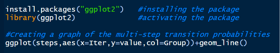
We, then, install and activate the “ggplot2” package, and plot the graph of the multi-step transition probabilities using the code:
We get our full and final output as:
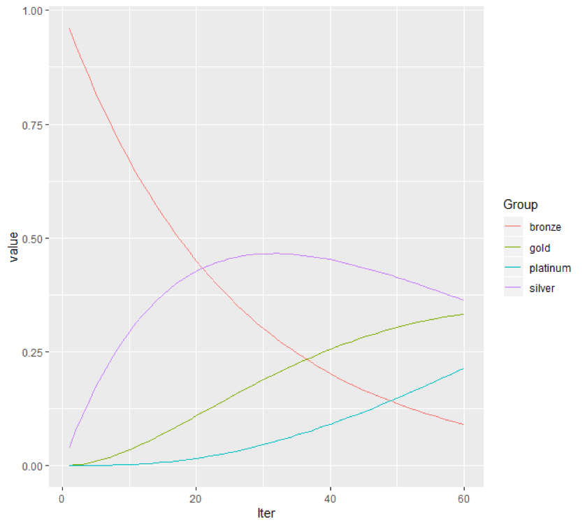
Some observations and conclusions that can be made from the above graph are:
- Clearly, the probability of remaining in state 0 is decreasing with time (as with time, passengers are travelling more and moving to other states)
- The probability of remaining in state 1, first rises, reaches a peak (inflexion point) at around month 32, and then starts falling as more and more passengers are moving to state 2 and state 3.
- Thus, the probability of being in state 2 and 3 clearly, keeps on increasing with time.
Well done!!! You have successfully completed the project. Hope, it was insightful and helpful to you!!!